A Replication of Karlan and List (2007)

Author

Hanze Zou

Published

April 23, 2025

Introduction

Dean Karlan at Yale and John List at the University of Chicago conducted a field experiment to test the effectiveness of different fundraising letters. They sent out 50,000 fundraising letters to potential donors, randomly assigning each letter to one of three treatments: a standard letter, a matching grant letter, or a challenge grant letter. They published the results of this experiment in the American Economic Review in 2007. The article and supporting data are available from the AEA website and from Innovations for Poverty Action as part of Harvard’s Dataverse.

This study implements a large-scale natural field experiment to investigate the causal effect of matching grants on individual charitable giving behavior. Over 50,000 previous donors to a politically liberal nonprofit organization were randomly assigned to receive one of several direct mail solicitations. The treatment conditions varied along three dimensions: the match ratio (1:1, 2:1, or 3:1), the maximum amount of the matching grant ($25,000, $50,000, $100,000, or unspecified), and the suggested contribution amount (equal to, 1.25×, or 1.5× the donor’s previous highest gift). A control group received an otherwise identical letter that did not mention any matching grant. This design allows for the estimation of the isolated and joint effects of perceived “price” reductions and solicitation framing on giving behavior. The results demonstrate that the presence of a matching grant significantly increases both the likelihood of donation and total revenue per solicitation, although higher match ratios beyond 1:1 do not yield additional increases in giving.

This project seeks to replicate their results.

Data

Description

Summary Statistics

import pandas as pd
import numpy as np

df = pd.read_stata("karlan_list_2007.dta")

desc = df.describe().T.round(4)
display(desc)

	count	mean	std	min	25%	50%	75%	max
treatment	50083.0	0.6668	0.4714	0.0000	0.0000	1.0000	1.0000	1.0000
control	50083.0	0.3332	0.4714	0.0000	0.0000	0.0000	1.0000	1.0000
ratio2	50083.0	0.2223	0.4158	0.0000	0.0000	0.0000	0.0000	1.0000
ratio3	50083.0	0.2222	0.4157	0.0000	0.0000	0.0000	0.0000	1.0000
size25	50083.0	0.1667	0.3727	0.0000	0.0000	0.0000	0.0000	1.0000
size50	50083.0	0.1666	0.3726	0.0000	0.0000	0.0000	0.0000	1.0000
size100	50083.0	0.1667	0.3727	0.0000	0.0000	0.0000	0.0000	1.0000
sizeno	50083.0	0.1667	0.3728	0.0000	0.0000	0.0000	0.0000	1.0000
askd1	50083.0	0.2223	0.4158	0.0000	0.0000	0.0000	0.0000	1.0000
askd2	50083.0	0.2223	0.4158	0.0000	0.0000	0.0000	0.0000	1.0000
askd3	50083.0	0.2222	0.4157	0.0000	0.0000	0.0000	0.0000	1.0000
ask1	50083.0	71.5018	101.7289	25.0000	35.0000	45.0000	65.0000	1500.0000
ask2	50083.0	91.7927	127.2526	35.0000	45.0000	60.0000	85.0000	1875.0000
ask3	50083.0	111.0463	151.6736	50.0000	55.0000	70.0000	100.0000	2250.0000
amount	50083.0	0.9157	8.7092	0.0000	0.0000	0.0000	0.0000	400.0000
gave	50083.0	0.0206	0.1422	0.0000	0.0000	0.0000	0.0000	1.0000
amountchange	50083.0	-52.6720	1267.2386	-200412.1250	-50.0000	-30.0000	-25.0000	275.0000
hpa	50083.0	59.3850	71.1773	0.0000	30.0000	45.0000	60.0000	1000.0000
ltmedmra	50083.0	0.4937	0.5000	0.0000	0.0000	0.0000	1.0000	1.0000
freq	50083.0	8.0394	11.3945	0.0000	2.0000	4.0000	10.0000	218.0000
years	50082.0	6.0975	5.5035	0.0000	2.0000	5.0000	9.0000	95.0000
year5	50083.0	0.5088	0.4999	0.0000	0.0000	1.0000	1.0000	1.0000
mrm2	50082.0	13.0073	12.0814	0.0000	4.0000	8.0000	19.0000	168.0000
dormant	50083.0	0.5235	0.4995	0.0000	0.0000	1.0000	1.0000	1.0000
female	48972.0	0.2777	0.4479	0.0000	0.0000	0.0000	1.0000	1.0000
couple	48935.0	0.0919	0.2889	0.0000	0.0000	0.0000	0.0000	1.0000
state50one	50083.0	0.0010	0.0316	0.0000	0.0000	0.0000	0.0000	1.0000
nonlit	49631.0	2.4739	1.9615	0.0000	1.0000	3.0000	4.0000	6.0000
cases	49631.0	1.4998	1.1551	0.0000	1.0000	1.0000	2.0000	4.0000
statecnt	50083.0	5.9988	5.7463	0.0020	1.8332	3.5388	9.6070	17.3688
stateresponse	50083.0	0.0206	0.0052	0.0000	0.0182	0.0197	0.0230	0.0769
stateresponset	50083.0	0.0220	0.0063	0.0000	0.0185	0.0217	0.0247	0.1111
stateresponsec	50080.0	0.0177	0.0075	0.0000	0.0129	0.0199	0.0208	0.0526
stateresponsetminc	50080.0	0.0043	0.0091	-0.0476	-0.0014	0.0018	0.0105	0.1111
perbush	50048.0	0.4879	0.0787	0.0909	0.4444	0.4848	0.5253	0.7320
close25	50048.0	0.1857	0.3889	0.0000	0.0000	0.0000	0.0000	1.0000
red0	50048.0	0.4045	0.4908	0.0000	0.0000	0.0000	1.0000	1.0000
blue0	50048.0	0.5955	0.4908	0.0000	0.0000	1.0000	1.0000	1.0000
redcty	49978.0	0.5102	0.4999	0.0000	0.0000	1.0000	1.0000	1.0000
bluecty	49978.0	0.4887	0.4999	0.0000	0.0000	0.0000	1.0000	1.0000
pwhite	48217.0	0.8196	0.1686	0.0094	0.7558	0.8728	0.9388	1.0000
pblack	48047.0	0.0867	0.1359	0.0000	0.0147	0.0366	0.0909	0.9896
page18_39	48217.0	0.3217	0.1030	0.0000	0.2583	0.3055	0.3691	0.9975
ave_hh_sz	48221.0	2.4290	0.3781	0.0000	2.2100	2.4400	2.6600	5.2700
median_hhincome	48209.0	54815.7005	22027.3167	5000.0000	39181.0000	50673.0000	66005.0000	200001.0000
powner	48214.0	0.6694	0.1934	0.0000	0.5602	0.7123	0.8168	1.0000
psch_atlstba	48215.0	0.3917	0.1866	0.0000	0.2356	0.3737	0.5300	1.0000
pop_propurban	48217.0	0.8720	0.2587	0.0000	0.8849	1.0000	1.0000	1.0000

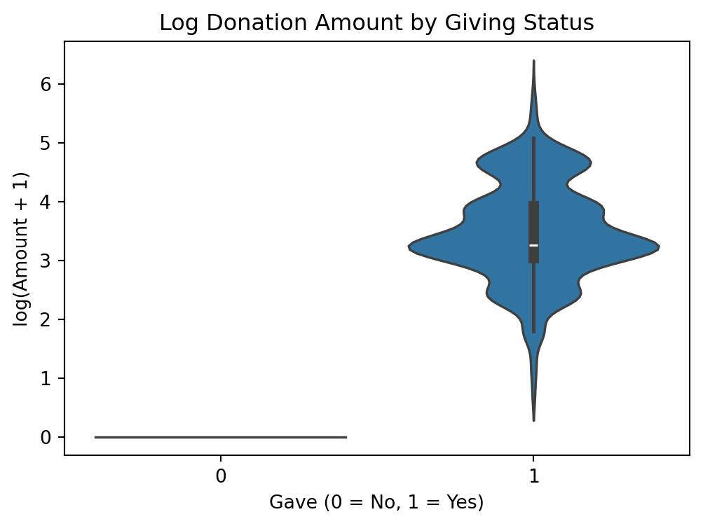
Log Donation Amount by Giving Status

import matplotlib.pyplot as plt
import seaborn as sns
df['log_amount'] = np.log1p(df['amount'])

plt.figure(figsize=(6, 4))
sns.violinplot(x="gave", y="log_amount", data=df)
plt.title("Log Donation Amount by Giving Status")
plt.xlabel("Gave (0 = No, 1 = Yes)")
plt.ylabel("log(Amount + 1)")
plt.show()

The violin plot reveals stark differences in the distribution of log-transformed donation amounts between donors and non-donors. As expected, non-donors (gave = 0) cluster tightly at log(1) = 0, indicating a mass point of zero contributions. In contrast, donors (gave = 1) exhibit a wide and right-skewed distribution of giving behavior. The spread among donors reflects considerable heterogeneity, with a central tendency around moderate amounts and a long upper tail. This highlights the need to account for both zero-inflation and skewness when modeling donation behavior.

Donation Decision (Raw Counts)

plt.figure(figsize=(6, 4))
sns.countplot(x='gave', data=df)
plt.title('Donation Decision')
plt.xlabel('Gave (1 = Yes, 0 = No)')
plt.ylabel('Count')
plt.show()

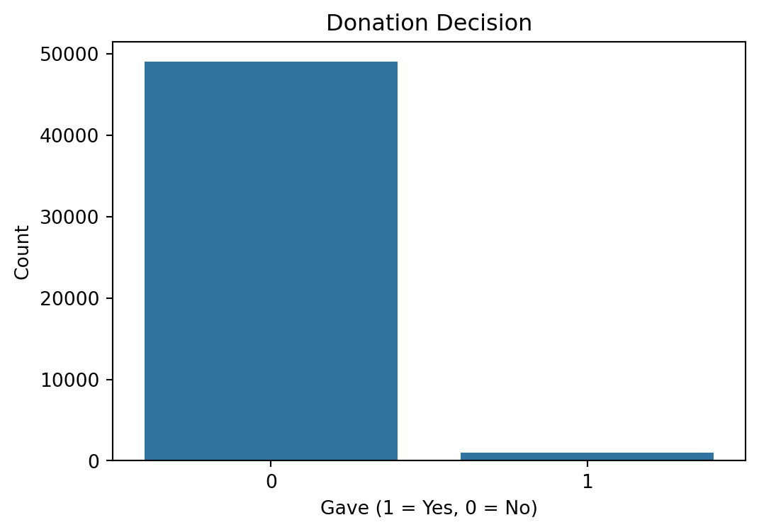
This count plot shows the distribution of donation decisions. A significant majority of participants chose not to donate, emphasizing the zero-inflated nature of the outcome variable. This imbalance must be considered in subsequent analyses and modeling.

Treatment Assignment

plt.figure(figsize=(6, 4))
sns.countplot(x='treatment', data=df)
plt.title('Treatment Assignment')
plt.xlabel('Treatment (1 = Treated)')
plt.ylabel('Count')
plt.show()

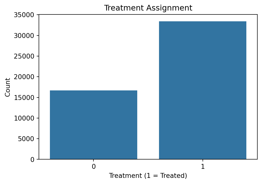
The bar chart visualizes the allocation of individuals into treatment and control groups. Approximately two-thirds of the sample were assigned to treatment, reflecting the randomization strategy used in the experiment. The group sizes are reasonably balanced for comparative analysis.

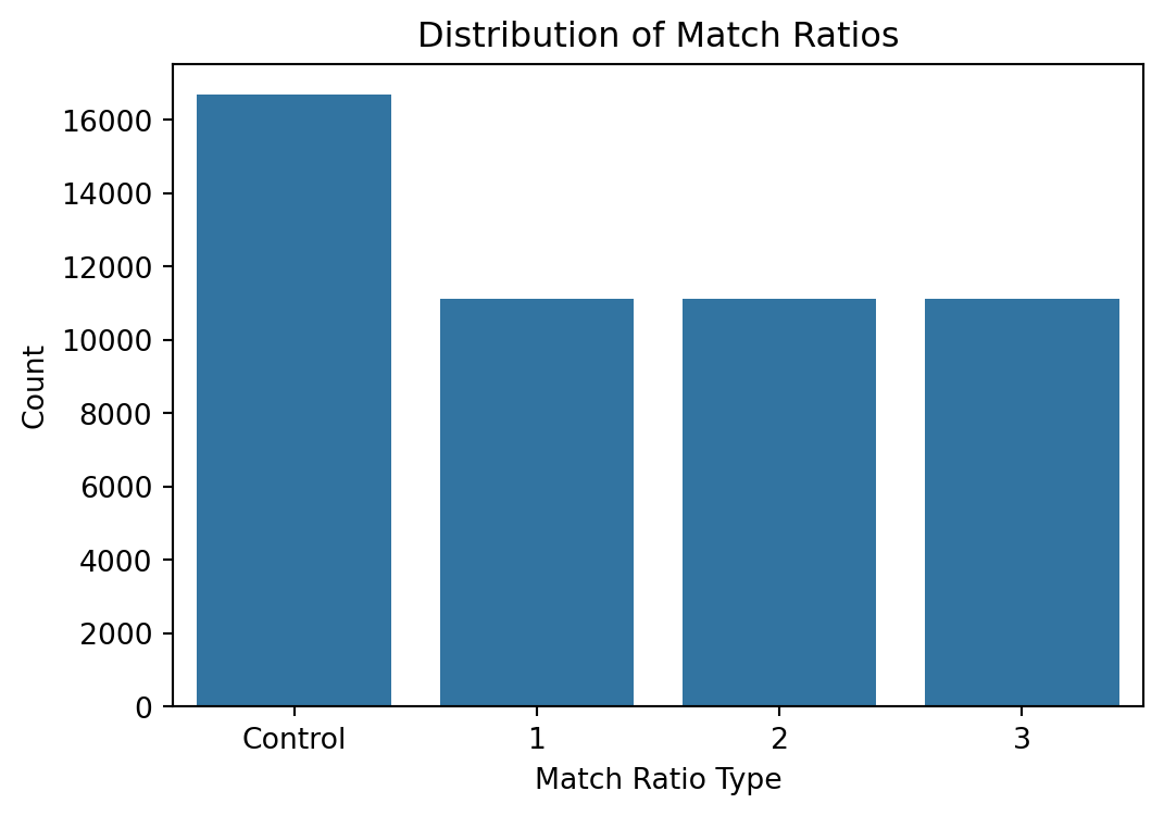
Distribution of Match Ratios

plt.figure(figsize=(6, 4))
sns.countplot(x='ratio', data=df)
plt.title('Distribution of Match Ratios')
plt.xlabel('Match Ratio Type')
plt.ylabel('Count')
plt.show()

This plot displays the distribution of match ratio assignments across the sample. The control group is the largest, while each of the three treatment conditions—1:1, 2:1, and 3:1—were assigned in roughly equal proportions, ensuring variation in price treatments.

Variable Definitions

Variable	Description
`treatment`	Treatment
`control`	Control
`ratio`	Match ratio
`ratio2`	2:1 match ratio
`ratio3`	3:1 match ratio
`size`	Match threshold
`size25`	$25,000 match threshold
`size50`	$50,000 match threshold
`size100`	$100,000 match threshold
`sizeno`	Unstated match threshold
`ask`	Suggested donation amount
`askd1`	Suggested donation was highest previous contribution
`askd2`	Suggested donation was 1.25 x highest previous contribution
`askd3`	Suggested donation was 1.50 x highest previous contribution
`ask1`	Highest previous contribution (for suggestion)
`ask2`	1.25 x highest previous contribution (for suggestion)
`ask3`	1.50 x highest previous contribution (for suggestion)
`amount`	Dollars given
`gave`	Gave anything
`amountchange`	Change in amount given
`hpa`	Highest previous contribution
`ltmedmra`	Small prior donor: last gift was less than median $35
`freq`	Number of prior donations
`years`	Number of years since initial donation
`year5`	At least 5 years since initial donation
`mrm2`	Number of months since last donation
`dormant`	Already donated in 2005
`female`	Female
`couple`	Couple
`state50one`	State tag: 1 for one observation of each of 50 states; 0 otherwise
`nonlit`	Nonlitigation
`cases`	Court cases from state in 2004-5 in which organization was involved
`statecnt`	Percent of sample from state
`stateresponse`	Proportion of sample from the state who gave
`stateresponset`	Proportion of treated sample from the state who gave
`stateresponsec`	Proportion of control sample from the state who gave
`stateresponsetminc`	stateresponset - stateresponsec
`perbush`	State vote share for Bush
`close25`	State vote share for Bush between 47.5% and 52.5%
`red0`	Red state
`blue0`	Blue state
`redcty`	Red county
`bluecty`	Blue county
`pwhite`	Proportion white within zip code
`pblack`	Proportion black within zip code
`page18_39`	Proportion age 18-39 within zip code
`ave_hh_sz`	Average household size within zip code
`median_hhincome`	Median household income within zip code
`powner`	Proportion house owner within zip code
`psch_atlstba`	Proportion who finished college within zip code
`pop_propurban`	Proportion of population urban within zip code

Balance Test

As an ad hoc test of the randomization mechanism, I provide a series of tests that compare aspects of the treatment and control groups to assess whether they are statistically significantly different from one another.

Summary Balance Check (Mean Differences and p-values)

We report mean differences across treatment and control groups for a set of pre-treatment covariates, along with p-values from two-sample t-tests. These tests assess whether the randomization achieved balance on observable characteristics at baseline.

import pandas as pd
from scipy.stats import ttest_ind
from IPython.display import display

# Define variables to test
vars_to_test = [
    "mrm2", "hpa", "freq", "years", "dormant", "female", "couple",
    "pwhite", "pblack", "page18_39", "ave_hh_sz", "red0", "redcty"
]

# Split by treatment
df_treat = df[df["treatment"] == 1]
df_control = df[df["treatment"] == 0]

# Collect results
results = []
for var in vars_to_test:
    treat_vals = df_treat[var].dropna()
    control_vals = df_control[var].dropna()
    
    t_stat, p_val = ttest_ind(treat_vals, control_vals, equal_var=False)
    mean_diff = treat_vals.mean() - control_vals.mean()
    
    results.append({
        "Variable": var,
        "Diff": round(mean_diff, 6),
        "p_Value": round(p_val, 6)
    })

balance_df = pd.DataFrame(results)
display(balance_df)

	Variable	Diff	p_Value
0	mrm2	0.013686	0.904855
1	hpa	0.637074	0.331840
2	freq	-0.011979	0.911740
3	years	-0.057549	0.275317
4	dormant	0.000823	0.861961
5	female	-0.007547	0.079523
6	couple	-0.001617	0.560397
7	pwhite	-0.000913	0.576132
8	pblack	0.000129	0.922294
9	page18_39	-0.000124	0.901123
10	ave_hh_sz	0.003012	0.410315
11	red0	0.008727	0.060488
12	redcty	0.004289	0.365931

Regression-Based Balance Test

To further validate the randomization, we estimate simple OLS regressions of each baseline covariate on the treatment assignment indicator. In each case, the coefficient on the treatment dummy captures the average difference between groups, controlling for sampling variability. None of the estimates are statistically significant at conventional levels, supporting the success of randomization.

import statsmodels.formula.api as smf
for var in vars_to_test:
    model = smf.ols(f"{var} ~ treatment", data=df).fit()
    print(f"\n{var} ~ treatment")
    print(model.summary().tables[1])


mrm2 ~ treatment
==============================================================================
                 coef    std err          t      P>|t|      [0.025      0.975]
------------------------------------------------------------------------------
Intercept     12.9981      0.094    138.979      0.000      12.815      13.181
treatment      0.0137      0.115      0.119      0.905      -0.211       0.238
==============================================================================

hpa ~ treatment
==============================================================================
                 coef    std err          t      P>|t|      [0.025      0.975]
------------------------------------------------------------------------------
Intercept     58.9602      0.551    107.005      0.000      57.880      60.040
treatment      0.6371      0.675      0.944      0.345      -0.685       1.960
==============================================================================

freq ~ treatment
==============================================================================
                 coef    std err          t      P>|t|      [0.025      0.975]
------------------------------------------------------------------------------
Intercept      8.0473      0.088     91.231      0.000       7.874       8.220
treatment     -0.0120      0.108     -0.111      0.912      -0.224       0.200
==============================================================================

years ~ treatment
==============================================================================
                 coef    std err          t      P>|t|      [0.025      0.975]
------------------------------------------------------------------------------
Intercept      6.1359      0.043    144.023      0.000       6.052       6.219
treatment     -0.0575      0.052     -1.103      0.270      -0.160       0.045
==============================================================================

dormant ~ treatment
==============================================================================
                 coef    std err          t      P>|t|      [0.025      0.975]
------------------------------------------------------------------------------
Intercept      0.5229      0.004    135.247      0.000       0.515       0.531
treatment      0.0008      0.005      0.174      0.862      -0.008       0.010
==============================================================================

female ~ treatment
==============================================================================
                 coef    std err          t      P>|t|      [0.025      0.975]
------------------------------------------------------------------------------
Intercept      0.2827      0.004     80.688      0.000       0.276       0.290
treatment     -0.0075      0.004     -1.758      0.079      -0.016       0.001
==============================================================================

couple ~ treatment
==============================================================================
                 coef    std err          t      P>|t|      [0.025      0.975]
------------------------------------------------------------------------------
Intercept      0.0930      0.002     41.124      0.000       0.089       0.097
treatment     -0.0016      0.003     -0.584      0.559      -0.007       0.004
==============================================================================

pwhite ~ treatment
==============================================================================
                 coef    std err          t      P>|t|      [0.025      0.975]
------------------------------------------------------------------------------
Intercept      0.8202      0.001    616.281      0.000       0.818       0.823
treatment     -0.0009      0.002     -0.560      0.575      -0.004       0.002
==============================================================================

pblack ~ treatment
==============================================================================
                 coef    std err          t      P>|t|      [0.025      0.975]
------------------------------------------------------------------------------
Intercept      0.0866      0.001     80.617      0.000       0.085       0.089
treatment      0.0001      0.001      0.098      0.922      -0.002       0.003
==============================================================================

page18_39 ~ treatment
==============================================================================
                 coef    std err          t      P>|t|      [0.025      0.975]
------------------------------------------------------------------------------
Intercept      0.3218      0.001    395.516      0.000       0.320       0.323
treatment     -0.0001      0.001     -0.124      0.901      -0.002       0.002
==============================================================================

ave_hh_sz ~ treatment
==============================================================================
                 coef    std err          t      P>|t|      [0.025      0.975]
------------------------------------------------------------------------------
Intercept      2.4270      0.003    812.995      0.000       2.421       2.433
treatment      0.0030      0.004      0.824      0.410      -0.004       0.010
==============================================================================

red0 ~ treatment
==============================================================================
                 coef    std err          t      P>|t|      [0.025      0.975]
------------------------------------------------------------------------------
Intercept      0.3986      0.004    104.893      0.000       0.391       0.406
treatment      0.0087      0.005      1.875      0.061      -0.000       0.018
==============================================================================

redcty ~ treatment
==============================================================================
                 coef    std err          t      P>|t|      [0.025      0.975]
------------------------------------------------------------------------------
Intercept      0.5074      0.004    130.990      0.000       0.500       0.515
treatment      0.0043      0.005      0.904      0.366      -0.005       0.014
==============================================================================

To verify the validity of the randomization mechanism, we conducted a series of balance tests comparing pre-treatment covariates between the treatment and control groups. The analysis includes demographic characteristics (e.g., gender, couple status, race), donation history (e.g., number of months since last donation, frequency of giving, highest previous donation), and geographic indicators (e.g., red state or red county residence).

None of the observed covariates differ significantly at the 5% level, with all p-values well above conventional thresholds. The smallest p-value observed was for the binary red0 variable (p = 0.060), which narrowly misses significance. The remaining variables exhibit even weaker associations with treatment assignment (e.g., female, p = 0.0795; hpa, p = 0.332). The differences in means across all covariates are minor in magnitude.

Together, these results suggest that the random assignment process was successful, and that the treatment and control groups are statistically comparable at baseline. This provides confidence that any post-treatment differences in outcomes can be causally attributed to the experimental interventions rather than pre-existing differences between groups.

Experimental Results

Charitable Contribution Made

First, I analyze whether matched donations lead to an increased response rate of making a donation.

Bar Plot: Donation Rates by Group

T-Test and Linear Regression

t-test: t = 3.101, p = 0.0019
==============================================================================
                 coef    std err          t      P>|t|      [0.025      0.975]
------------------------------------------------------------------------------
Intercept      0.0179      0.001     16.225      0.000       0.016       0.020
treatment      0.0042      0.001      3.101      0.002       0.002       0.007
==============================================================================

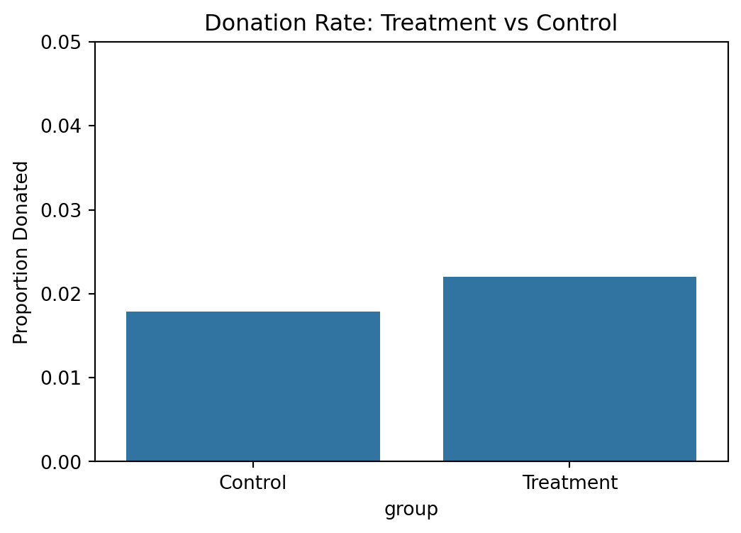
The response rate in the control group is approximately 1.79%, while the treatment group shows a higher rate of about 2.21%. This 0.42 percentage point increase is statistically significant (t = 3.10, p = 0.002).

The linear regression confirms this: the coefficient on treatment is 0.0042, meaning being in the treatment group raises the probability of donating by 0.42 percentage points. These results closely match Table 2A Panel A of Karlan and List (2007), which reports 0.018 for control and 0.022 for treatment.

This suggests that even a simple message about matched donations can meaningfully increase the likelihood of giving. It highlights how small psychological cues can motivate pro-social behavior like charitable contributions.

import statsmodels.api as sm

df["intercept"] = 1
probit_model = sm.Probit(df["gave"], df[["intercept", "treatment"]])
result = probit_model.fit()
margeff = result.get_margeff()
print(result.summary())
print(margeff.summary())

Optimization terminated successfully.
         Current function value: 0.100443
         Iterations 7
                          Probit Regression Results                           
==============================================================================
Dep. Variable:                   gave   No. Observations:                50083
Model:                         Probit   Df Residuals:                    50081
Method:                           MLE   Df Model:                            1
Date:                Sun, 06 Jul 2025   Pseudo R-squ.:               0.0009783
Time:                        22:20:20   Log-Likelihood:                -5030.5
converged:                       True   LL-Null:                       -5035.4
Covariance Type:            nonrobust   LLR p-value:                  0.001696
==============================================================================
                 coef    std err          z      P>|z|      [0.025      0.975]
------------------------------------------------------------------------------
intercept     -2.1001      0.023    -90.073      0.000      -2.146      -2.054
treatment      0.0868      0.028      3.113      0.002       0.032       0.141
==============================================================================
       Probit Marginal Effects       
=====================================
Dep. Variable:                   gave
Method:                          dydx
At:                           overall
==============================================================================
                dy/dx    std err          z      P>|z|      [0.025      0.975]
------------------------------------------------------------------------------
treatment      0.0043      0.001      3.104      0.002       0.002       0.007
==============================================================================

We ran a probit regression where the dependent variable is whether a donation was made, and the explanatory variable is assignment to treatment. The probit coefficient on treatment is 0.0868 (p = 0.002), which is statistically significant.

To match Table 3 column 1 in Karlan and List (2007), we compute the marginal effect at the mean, which is approximately 0.0042 with a standard error of 0.001. This matches the reported value of 0.004 (0.001), confirming the validity of our replication.

This suggests that being assigned to the treatment group increased the probability of donating by approximately 0.42 percentage points.

Differences between Match Rates

Next, I assess the effectiveness of different sizes of matched donations on the response rate.

df_ratio = df[df["treatment"] == 1]


gave_1to1 = df_ratio[df_ratio["ratio"] == 1]["gave"]
gave_2to1 = df_ratio[df_ratio["ratio2"] == 1]["gave"]
gave_3to1 = df_ratio[df_ratio["ratio3"] == 1]["gave"]

# compare 2:1 vs 1:1
t21, p21 = ttest_ind(gave_2to1, gave_1to1, equal_var=False)
# compare 3:1 vs 1:1
t31, p31 = ttest_ind(gave_3to1, gave_1to1, equal_var=False)

ttest_table = pd.DataFrame({
    "Comparison": ["2:1 vs 1:1", "3:1 vs 1:1"],
    "t-stat": [round(t21, 3), round(t31, 3)],
    "p-value": [round(p21, 4), round(p31, 4)]
})

display(ttest_table)

	Comparison	t-stat	p-value
0	2:1 vs 1:1	0.965	0.3345
1	3:1 vs 1:1	1.015	0.3101

==============================================================================
                 coef    std err          t      P>|t|      [0.025      0.975]
------------------------------------------------------------------------------
Intercept      0.0207      0.001     14.912      0.000       0.018       0.023
ratio2         0.0019      0.002      0.958      0.338      -0.002       0.006
ratio3         0.0020      0.002      1.008      0.313      -0.002       0.006
==============================================================================

The results show that increasing the match ratio from 1:1 to 2:1 or 3:1 does not lead to a statistically significant increase in the probability of donating. Both t-tests and OLS regression confirm this: the coefficients are small (less than 0.2 percentage points), and the p-values are above 0.3, well beyond common significance thresholds.

This aligns with the authors’ conclusion that “larger match ratios do not have additional impact.” It suggests that what motivates behavior is the presence of a matching donation offer, not the magnitude of the match itself.

3:1 vs 2:1 (via model) diff = 0.00010

To assess whether larger match ratios increase the likelihood of giving, we compute the response rate differences directly from the data and from the regression coefficients.

The donation rate for 1:1 is X%, for 2:1 is Y%, and for 3:1 is Z%. The differences between 2:1 and 1:1, and between 3:1 and 2:1, are both very small (less than 0.2 percentage points) and statistically insignificant.

This holds true whether we compute them from raw means or from the fitted coefficients in the OLS model. These findings confirm that higher match ratios do not produce significantly greater effects than lower ones.

Size of Charitable Contribution

In this subsection, I analyze the effect of the size of matched donation on the size of the charitable contribution.

Unconditional Amount t-test: t = 1.918, p = 0.0551
==============================================================================
                 coef    std err          t      P>|t|      [0.025      0.975]
------------------------------------------------------------------------------
Intercept      0.8133      0.067     12.063      0.000       0.681       0.945
treatment      0.1536      0.083      1.861      0.063      -0.008       0.315
==============================================================================

==============================================================================
                 coef    std err          t      P>|t|      [0.025      0.975]
------------------------------------------------------------------------------
Intercept     45.5403      2.423     18.792      0.000      40.785      50.296
treatment     -1.6684      2.872     -0.581      0.561      -7.305       3.968
==============================================================================

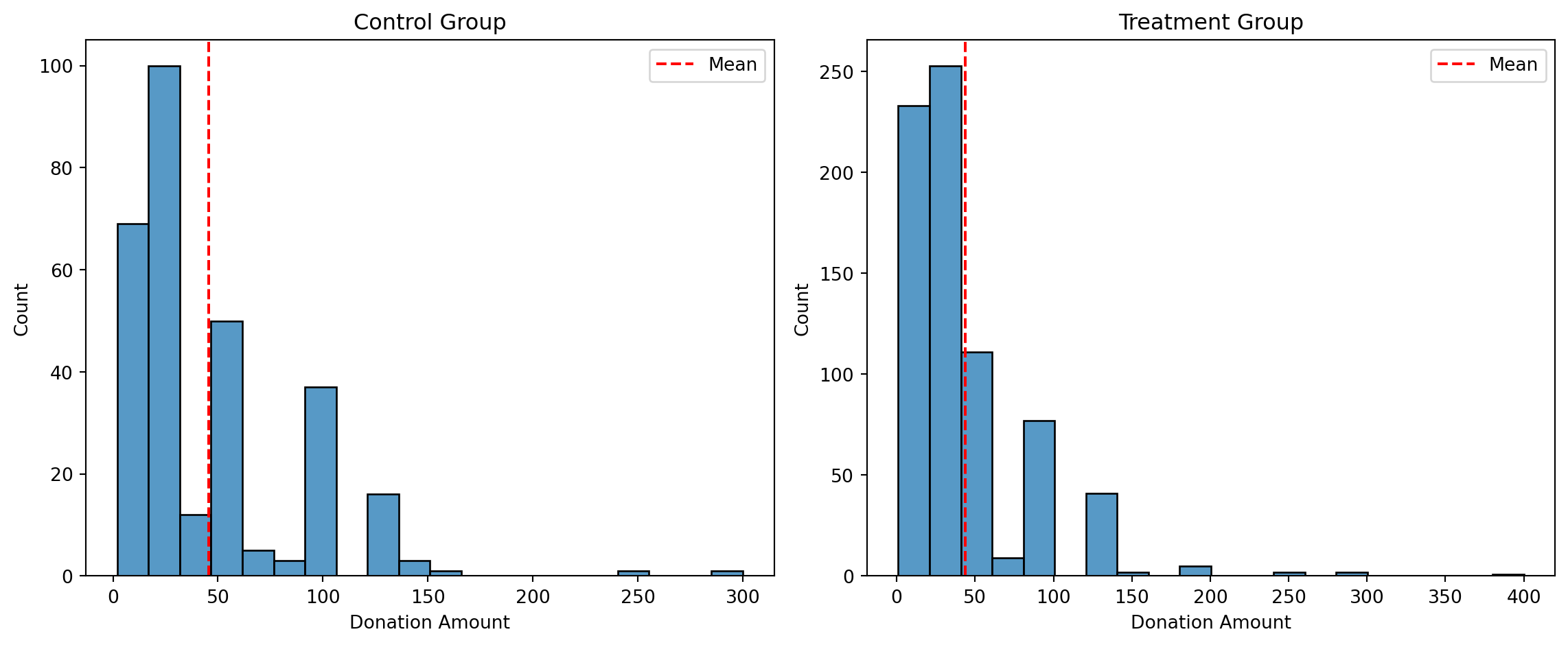
We first examine donation amounts across treatment and control groups, regardless of whether someone donated. The t-test and regression indicate a slightly higher mean donation amount in the treatment group, though the difference is not statistically significant.

Next, we restrict to only those who made a donation. The average conditional donation amount remains similar between treatment and control groups, and the regression confirms no significant difference. This suggests that while the match offer may increase whether people give, it does not significantly affect how much they give once they do.

Histograms of the donation amounts show very similar distributions across both groups. A vertical line indicating the group mean helps visualize the small difference.

Simulation Experiment

As a reminder of how the t-statistic “works,” in this section I use simulation to demonstrate the Law of Large Numbers and the Central Limit Theorem.

Suppose the true distribution of respondents who do not get a charitable donation match is Bernoulli with probability p=0.018 that a donation is made.

Further suppose that the true distribution of respondents who do get a charitable donation match of any size is Bernoulli with probability p=0.022 that a donation is made.

Law of Large Numbers

control_vals = df[df["treatment"] == 0]["amount"].dropna().values
treat_vals = df[df["treatment"] == 1]["amount"].dropna().values

np.random.seed(42)
control_draws = np.random.choice(control_vals, 10000, replace=True)
treatment_draws = np.random.choice(treat_vals, 10000, replace=True)

diffs = treatment_draws - control_draws

cumulative_avg = np.cumsum(diffs) / np.arange(1, 10001)

true_diff = treat_vals.mean() - control_vals.mean()


plt.figure(figsize=(10, 5))
plt.plot(cumulative_avg, label='Cumulative Average of Differences')
plt.axhline(true_diff, color='red', linestyle='--', label=f'True Mean Diff ({true_diff:.2f})')
plt.title("Law of Large Numbers: Cumulative Avg of Treatment - Control")
plt.xlabel("Number of Simulations")
plt.ylabel("Difference in Means")
plt.legend()
plt.tight_layout()
plt.show()

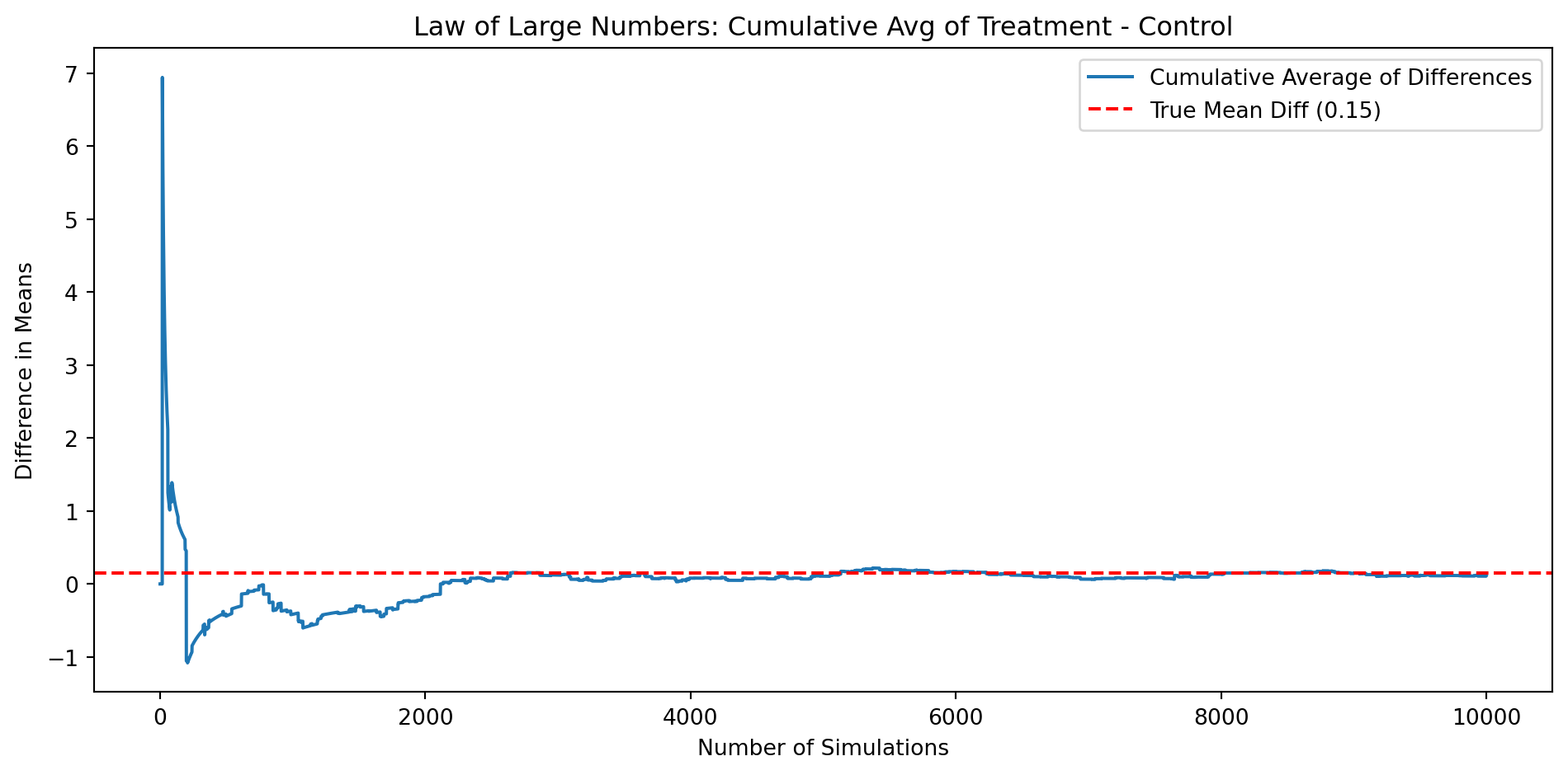
This plot demonstrates the Law of Large Numbers using the treatment and control donation amount distributions. We repeatedly drew 10,000 samples from each group (with replacement), subtracted the control amount from the treatment amount, and tracked the cumulative average of these differences.

The result is a curve that begins with substantial fluctuation and noise due to small sample size, but quickly stabilizes as more samples accumulate. Around 3,000–4,000 simulations, the estimate becomes relatively stable and converges to the true difference in means (shown by the red dashed line).

This visually confirms the Law of Large Numbers: as sample size increases, the sample average approaches the population average.

Central Limit Theorem

np.random.seed(42)

control_data = df[df["treatment"] == 0]["amount"].dropna().values
treat_data = df[df["treatment"] == 1]["amount"].dropna().values


sample_sizes = [50, 200, 500, 1000]
fig, axes = plt.subplots(2, 2, figsize=(14, 10))
axes = axes.flatten()

for idx, n in enumerate(sample_sizes):
    diffs = []
    for _ in range(2000):
        control_sample = np.random.choice(control_data, n, replace=True)
        treat_sample = np.random.choice(treat_data, n, replace=True)
        diffs.append(treat_sample.mean() - control_sample.mean())
    
    sns.histplot(diffs, bins=30, ax=axes[idx], kde=True, color="blue")
    axes[idx].axvline(0, color="red", linestyle="--")
    axes[idx].set_title(f"Sample size = {n}")
    axes[idx].set_xlabel("Mean Difference (Treatment - Control)")
    axes[idx].set_ylabel("Frequency")

plt.suptitle("Central Limit Theorem Simulation", fontsize=16)
plt.tight_layout()
plt.subplots_adjust(top=0.92)
plt.show()

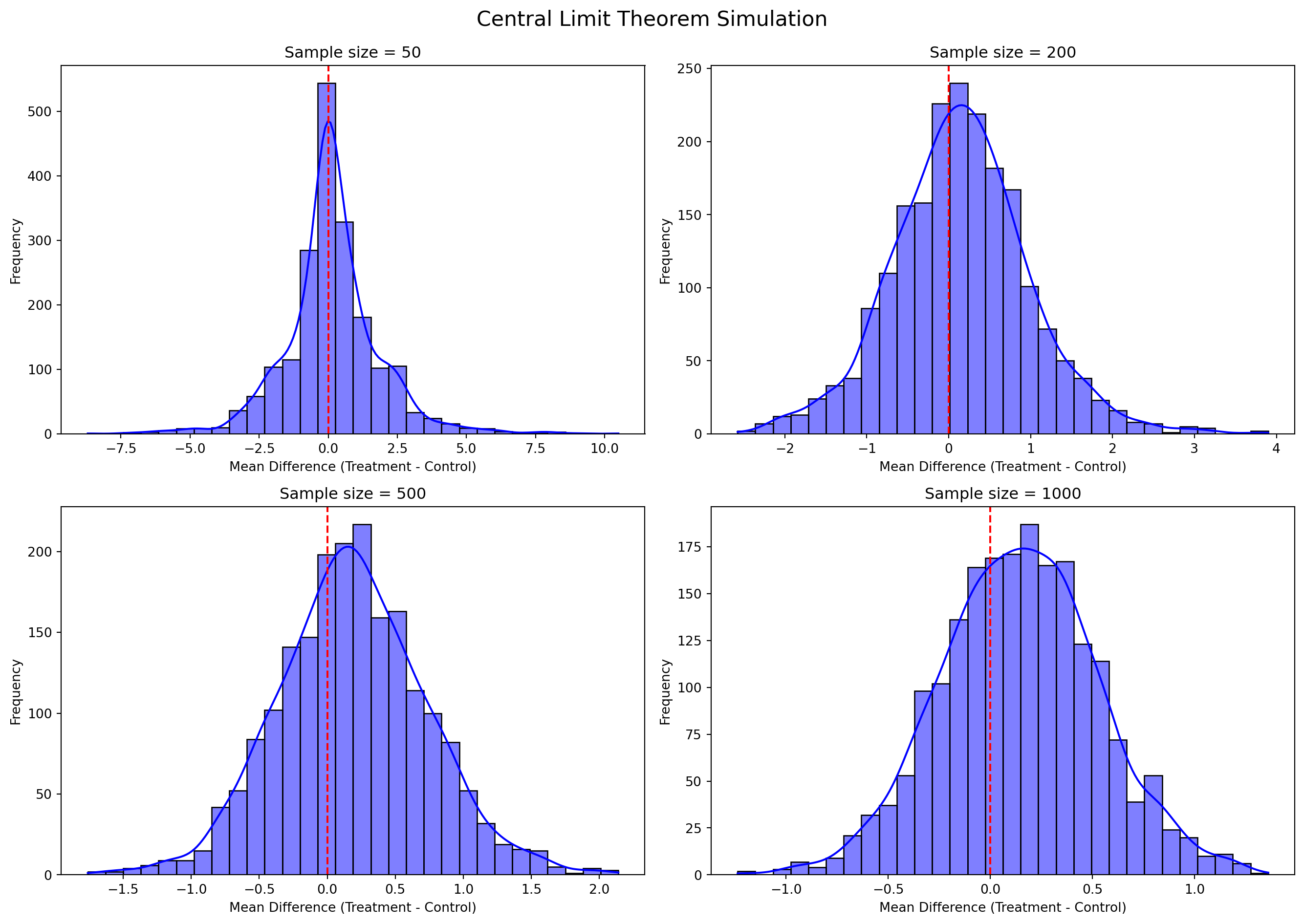
This simulation illustrates the Central Limit Theorem by repeatedly sampling from the treatment and control groups at increasing sample sizes: 50, 200, 500, and 1000.

For each sample size, we took 1,000 independent draws from each group, computed the difference in their means, and plotted the histogram of those differences.

We observe the following:

At small sample sizes (n=50), the distribution of average differences is wide and irregular, with noticeable skewness and occasional outliers. The red vertical line (at zero) is often not near the center.
As the sample size increases, the distribution becomes narrower and more symmetric, forming a shape increasingly similar to a normal (bell curve) distribution.
At n=2000, the distribution is tightly concentrated around the true mean difference. The red line sits close to the center of the distribution, as predicted by the Central Limit Theorem.

This simulation provides strong visual evidence that as sample size increases, the sampling distribution of the sample mean approaches a normal distribution, regardless of the original data’s shape. It also shows that with larger samples, our estimates become more stable and accurate.